library(survival)
breastcancer <- read.csv("https://raw.githubusercontent.com/anlane611/datasets/main/breastcancer.csv", row.names = 1)
attach(breastcancer)11.2: The Cox Proportional Hazards Model
Learning objectives
Define the Hazard function
Describe the proportional hazards assumption
Fit a Cox proportional hazards model in R
Classwise videos
If you have questions as you watch the videos, feel free to send me an email or slack message! I will address common questions at the beginning of class.
Textbook
ISLR 11.5
Application exercise
For this exercise, we will use the breast cancer data used in the first survival analysis lecture.
Code book:
| Variable | Description |
|---|---|
| pid | patient identifier |
| age | age, years |
| meno | menopausal status (0=premenopausal, 1=postmenopausal) |
| size | tumor size, mm |
| grade | tumor grade |
| nodes | number of positive lymph nodes |
| pgr | progesterone receptors (fmol/l) |
| er | estrogen receptors (fmol/l) |
| hormon | hormonal therapy (0=no, 1=yes) |
| rfstime | recurrence-free survival time |
| status | 0=alive w/o recurrence, 1=recurrence or death |
First, get a glimpse of the data and calculate some summary statistics. For example, what percentage of observations are censored?
Use the code below to generate Kaplan-Meier curves and perform the log-rank test.
#Kaplan-Meier curve for all patients
surv.fit <- survfit(Surv(rfstime,status)~1)
plot(surv.fit, xlab="Days", ylab="Estimated probability of survival")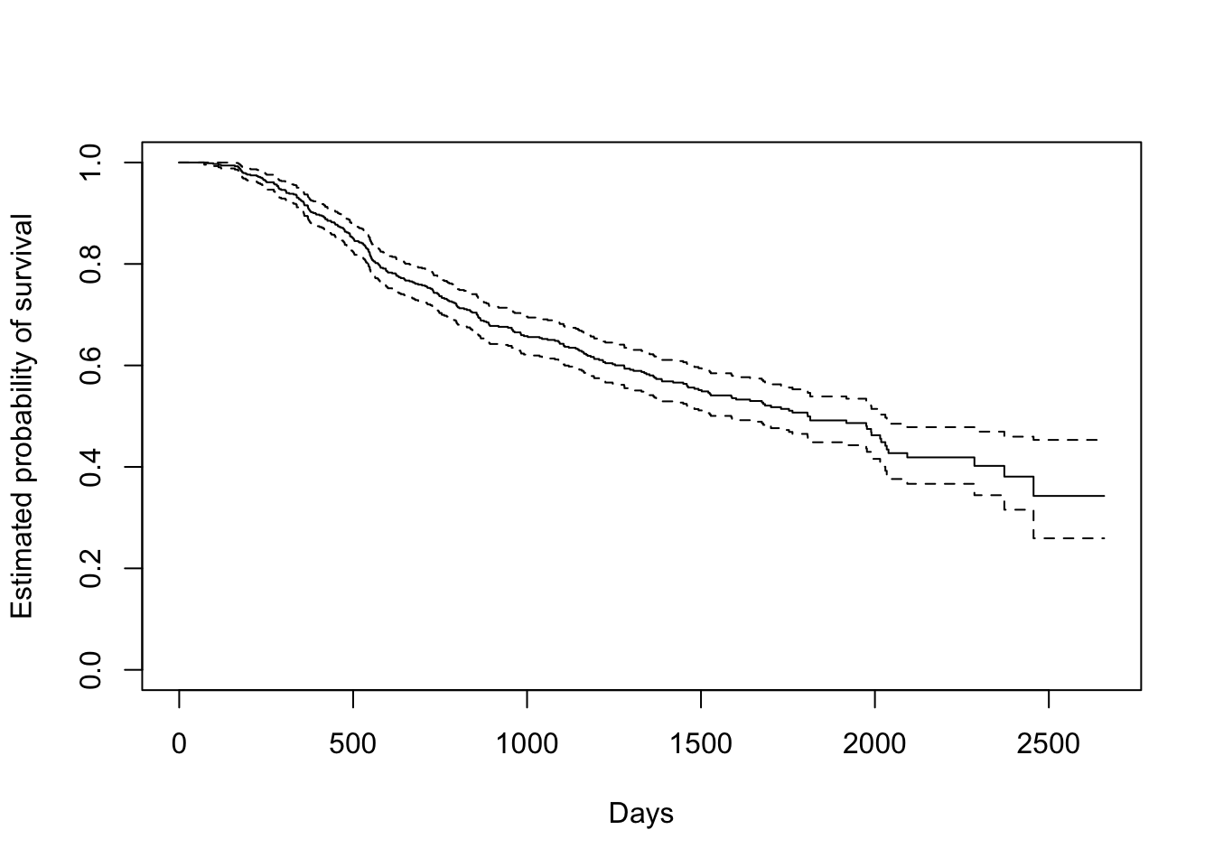
#Kaplan-Meier curve by treatment group
surv.fit.trt <- survfit(Surv(rfstime, status) ~ factor(hormon))
plot(surv.fit.trt, xlab="Days", ylab="Estimated probability of survival",
     col=c(2,4))
legend("topright", c("Trt", "No Trt"), col=c(4,2), lty=1)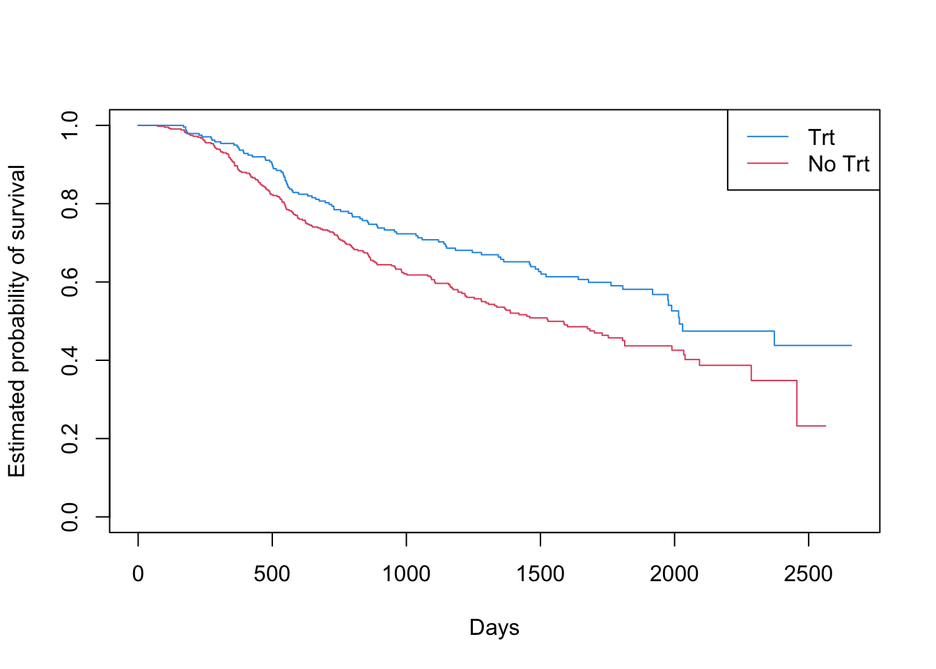
#Log-rank test
survdiff(Surv(rfstime, status) ~ factor(hormon))
Call:
survdiff(formula = Surv(rfstime, status) ~ factor(hormon))
N Observed Expected (O-E)^2/E (O-E)^2/V
factor(hormon)=0 440 205 180 3.37 8.56
factor(hormon)=1 246 94 119 5.12 8.56
Chisq= 8.6 on 1 degrees of freedom, p= 0.003 Now, let’s fit a Cox proportional hazards model. Let’s start by just using the main predictor of interest, hormone therapy treatment. We can use the coxph function in the survival package to fit the model.
fit.cox <- coxph(Surv(rfstime, status) ~ factor(hormon))
summary(fit.cox)
Call:
coxph(formula = Surv(rfstime, status) ~ factor(hormon))
n= 686, number of events= 299
coef exp(coef) se(coef) z Pr(>|z|)
factor(hormon)1 -0.3640 0.6949 0.1250 -2.911 0.0036 **
---
Signif. codes: 0 '***' 0.001 '**' 0.01 '*' 0.05 '.' 0.1 ' ' 1
exp(coef) exp(-coef) lower .95 upper .95
factor(hormon)1 0.6949 1.439 0.5438 0.8879
Concordance= 0.543 (se = 0.014 )
Likelihood ratio test= 8.82 on 1 df, p=0.003
Wald test = 8.47 on 1 df, p=0.004
Score (logrank) test = 8.57 on 1 df, p=0.003Examine the summary output for the model with only hormonal treatment group as a predictor.
What are the meanings and values of n and number of events?
How does the p-value of the hormonal treatment variable compare to the p-value obtained from the log-rank test?
Note that the exponentiated value of the coefficient estimate is already provided in the summary output. We can interpret exp(coef)=0.7 by saying the risk of death/recurrence for the treatment group is 30% lower than the risk of death/recurrence for the non-experimental treatment group.
Calculate the mean survival time for each treatment group without considering censoring. What is the difference between the groups and how does this compare to the results obtained with the model?
Recall that the Cox model relies on the key assumption of proportional hazards: the ratio of hazards is constant over time. Let’s check this assumption for the model. We can do this using the cox.zph function in the survival package. This generates a p-value for each predictor to test the proportional hazards assumption. A significant p-value here indicates that the assumption may be violated.
The GLOBAL line performs a test for the full model. Here, since we only have one predictor, the global test is the same as the predictor test.
test.ph <- cox.zph(fit.cox)
test.ph
chisq df p
factor(hormon) 0.227 1 0.63
GLOBAL 0.227 1 0.63We can also look at a plot of the Schoenfeld Residuals, which are a residual measure unique to survival models that are commonly used to test the proportional hazards assumption. A straight line indicates proportional hazards. Here, we see a fairly straight line with some veering off at later time points.
plot(test.ph)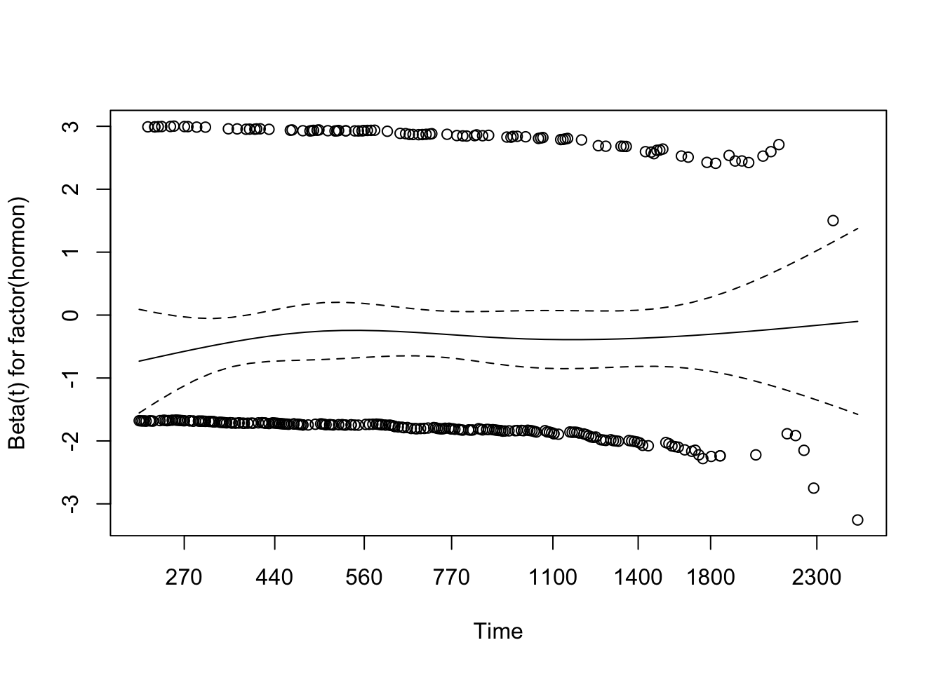
Now, add a few predictors to the model that you think are most relevant to accurately assess the relationship between treatment and survival time.
Fit the model and interpret the coefficient estimates. Which predictor(s) are statistically significant? Controlling for the other predictors, is there still a significant relationship between hormonal treatment group and survival time?
Use the cox.zph function to assess the proportional hazards assumption.
Additional practice
Labs in ISLR section 11.8