library(tidyverse)
population <- read.csv("https://raw.githubusercontent.com/anlane611/datasets/main/population.csv", header=TRUE)Homework 2
Due: Sunday, Sept 21st 11:59 PM
Using the provided Qmd template, complete the following exercises and submit the document with your answers on Gradescope, which you can access through Canvas. You must show your work for all problems.
Let \(X_1,X_2,...,X_n \stackrel {iid}{\sim} N(\mu,1)\), and recall the Normal PDF: \(f(x)=\frac{1}{\sqrt{2\pi\sigma^2 }} e^{\frac{-(x-\mu)^2 }{2\sigma^2} }\)
a. Write the likelihood function \(L(\mu)\)
b. Write the log-likelihood function \(l(\mu)\)
c. Find the maximum likelihood estimator of \(\mu\)
d. Determine if the MLE \(\hat{\mu}\) is an unbiased estimator of \(\mu\)
- In this exercise, you will conduct a simulation in R to evaluate the effect of sample size and sampling scheme on the sampling distribution of the mean.
We will use the dataset provided below to conduct the simulation. The dataset contains 100000 observations, so we will treat this as our population of interest. The dataset has 3 variables: 1 continuous variable (Y) and 2 categorical variables (X1 and X2).
First, let’s understand our population. Our main variable of interest will be Y.
What is the mean of Y? This will be our true parameter value, \(\mu\).
What is the mean of Y for each level of X2? How many observations are in each level of X2?
The code below simulates the sampling distribution of the mean if the data are collected using simple random sampling, where each member of the population has the same probability of being selected. Each sample is of size 100, and we will take 1000 different samples to understand the sampling distribution.
SRSmeans <- data.frame(means=NA) #create an empty dataframe to store the sample means
for(i in 1:1000){
  set.seed(i) #ensure that we have a different sample each time
  SRS.sample <- population |> slice(sample(1:n(),size=100)) #the slice function selects rows of the specified data (population), and the sample function randomly selects 100 numbers out of the sequence 1:100000
  SRSmeans[i,1] <- SRS.sample |> summarise(mean(Y)) #calculate the mean of each sample
}

ggplot(SRSmeans, aes(x=means)) +
  geom_histogram()+
  labs(title="Sampling distribution of the mean under simple random sampling")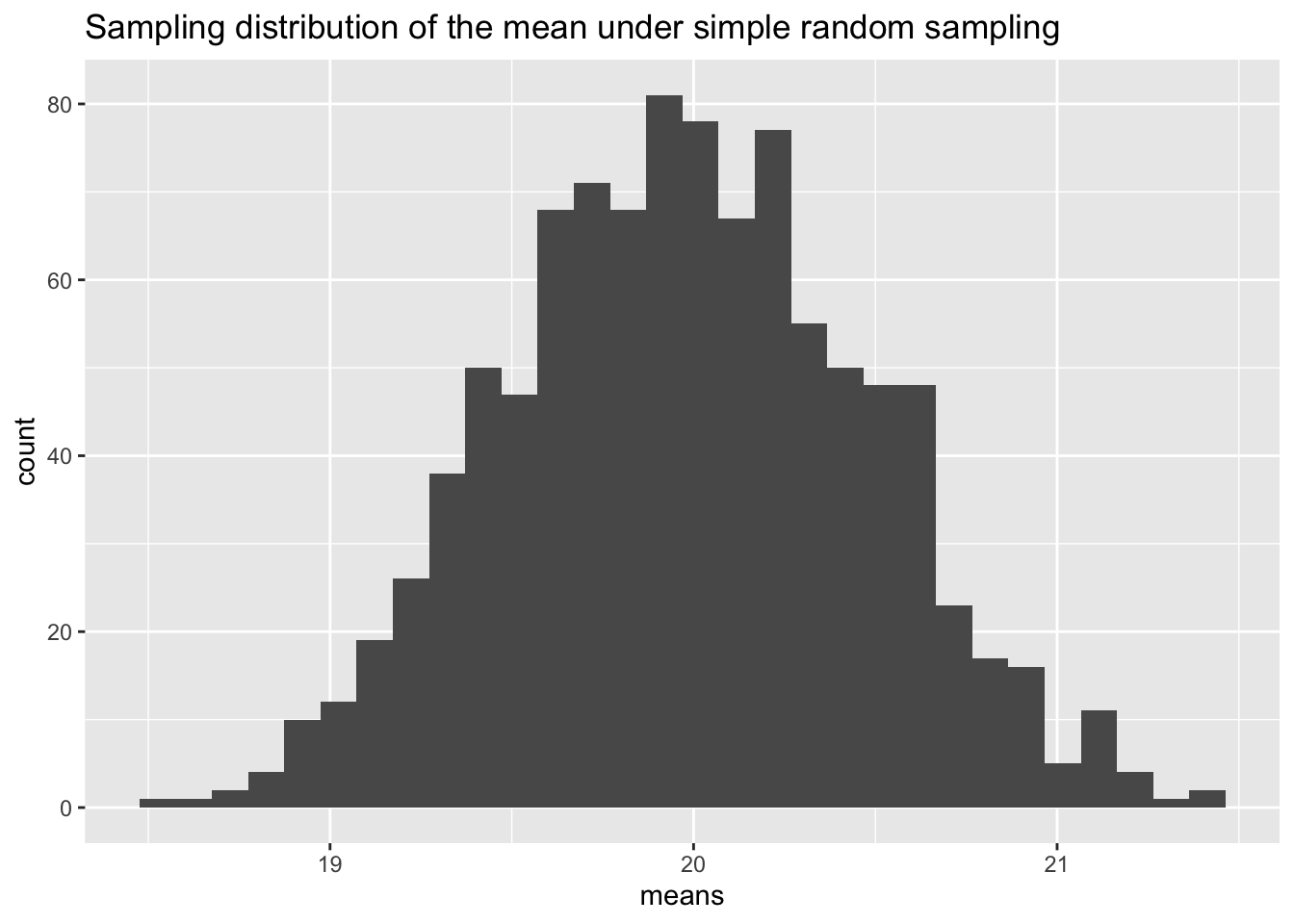
Does the histogram show an approximately normal distribution? What is its mean and how does it compare to the population mean?
Change the sample size of each sample from 100 to 10. Does the sampling distribution change in i) shape, ii) mean, and/or iii) spread compared to part c?
Next, we will explore the sampling distribution of the sample mean of Y under stratified sampling, where simple random samples are taken within subgroups. Here, we will use X2 as the group variable.
Fill in the two blanks in the code below to simulate the sampling distribution of the sample mean under stratified sampling for samples of size 100.
Stratmeans <- data.frame(means=NA) #create an empty dataframe to store the sample means
for(i in 1:1000){
  set.seed(i) #ensure that we have a different sample each time
  Stratified.sample <- population |>
                        group_by(__) |>
                        slice(sample(1:n(),size=50)) |>
                        ungroup()
  Stratmeans[i,1] <- Stratified.sample |> summarise(____(Y)) #calculate the mean of each sample
}

ggplot(Stratmeans, aes(x=means)) +
  geom_histogram()+
  labs(title="Sampling distribution of the mean under stratified sampling")
Does the histogram show an approximately normal distribution? What is its mean and how does it compare to the population mean?
Using your answers to parts b and f, what can you conclude about how sampling scheme can affect the sampling distribution of the mean?
Bonus: Simulate the sampling distribution under stratified sampling using X1 as the group variable. Start by calculating the sample size of each stratum and the true mean of Y in each stratum. Describe what you observe with the sampling distribution, how it compares to the sampling distribution you simulated in part e, and what this means for sampling scheme and sampling distributions.