Rows: 50
Columns: 3
$ family_income <dbl> 92.922, 0.250, 53.092, 50.200, 137.613, 47.957, 113.534,…
$ gift_aid      <dbl> 21.720, 27.470, 27.750, 27.220, 18.000, 18.520, 13.000, …
$ price_paid <dbl> 14.280, 8.530, 14.250, 8.780, 24.000, 23.480, 23.000, 29…Simple Linear Regression
Motivating example
A random sample of 50 students’ gift aid for students at Elmhurst College in 2011.
Research Question: What is the relationship between family income and price the student pays (total tuition - gift aid)?
Scatter plot of family income and price paid
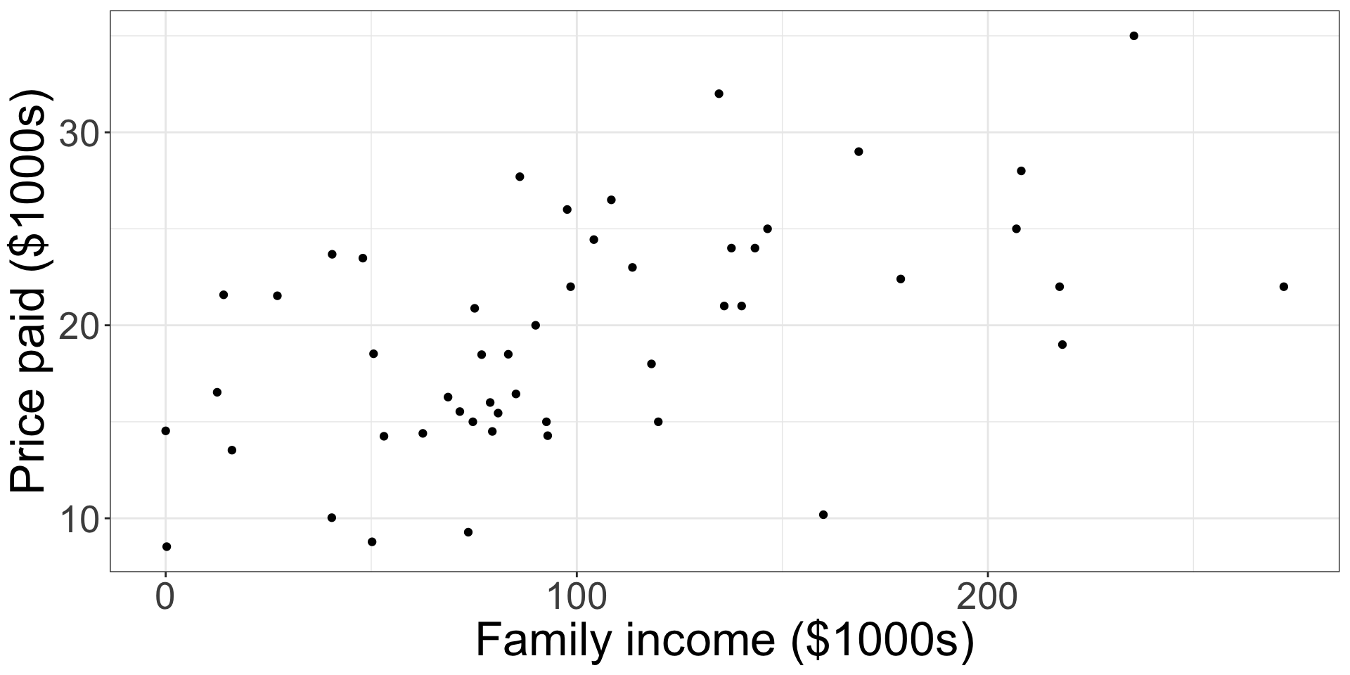
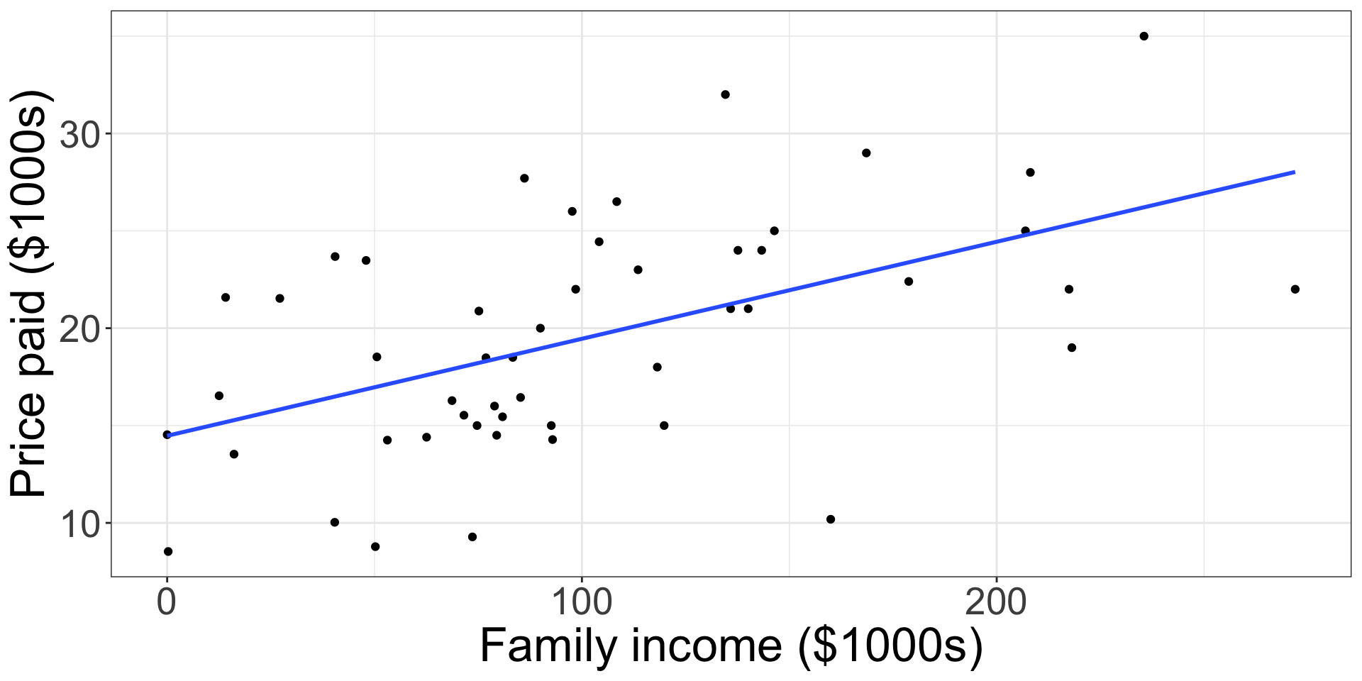
We want a “line of best fit” to characterize the relationship between the two (continuous) variables
Simple linear regression model
We define the simple linear regression model as:
\[ Y = \beta_0 + \beta_1X + \epsilon, \epsilon \sim N(0,\sigma^2) \]
We can also write this as:
\[ Y \sim N(\beta_0 + \beta_1X, \sigma^2) \]
Exercise
Label each component of the model with one of the following terms: random variable, fixed variable, parameter
Obtaining the estimates
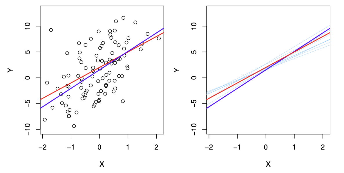
We use least squares estimation determine the “best” estimated values of \(\beta_0\) and \(\beta_1\)
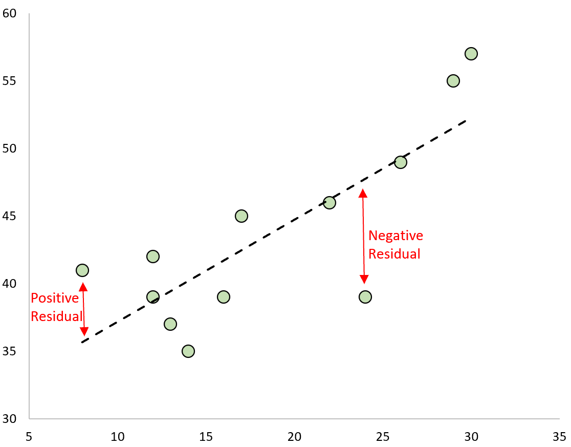
We will minimize the sum of squared residuals:
\(\sum_i (y_i - (\beta_0+\beta_1x_i))^2\)
Estimated regression line
We write the estimated regression line as:
\[ \hat{Y}=\hat{\beta_0}+\hat{\beta_1}X \]
and write the residuals \(r\) (\(\hat{e}\)) as \(r=Y-\hat{Y}\)
Exercise
Use the output below to write the estimated regression line for the elmhurst data
Standard error of the estimates
Hypothesis testing for coefficient estimates
\[H_0: \beta_1 = \]
\[ \frac{\hat{\beta_1}}{SE(\hat{\beta_1})} \sim t_{n-2} \]
Confidence Interval
Similarly, we can use the t-distribution to calculate the confidence interval, or a plausible range for the true value of the population parameter \(\beta_1\)
\[ \hat{\beta_1} \pm t^*_{n-2}[SE(\hat{\beta_1})] \]
Interpreting the results
                 Estimate Std. Error   t value     Pr(>|t|)
(Intercept)   14.47313102 1.38684598 10.436005 6.148375e-14
family_income 0.04982691 0.01160794 4.292486 8.530168e-05 2.5 % 97.5 %
(Intercept) 11.68469028 17.26157176
family_income 0.02648759 0.07316623
For each additional $1000 of family income, price paid in $1000s increases by 0.05, or $50, on average. The association between family income and price paid is statistically significant (p<.001, 95% CI: [0.03,0.07])
Interpreting the p-value and confidence interval individually
Assuming there is no association between family income and price paid, the probability of observing results as extreme as these is <.001. Therefore, we have evidence that there is a relationship between family income and price paid.
If we repeated this experiment 100 times and constructed a confidence interval in the same way each time, we would expect 95 of the intervals to contain the true value of \(\beta_1\). Therefore, we are 95% confident that the true value of \(\beta_1\) is between 0.03 and 0.07.
Exercise
Fit a model to assess the relationship between family income and gift aid. Write the fitted model and interpret the results.
elmhurst_slr_gift <- lm(gift_aid ~ family_income, data=elmhurst)
summary(elmhurst_slr_gift)$coefficients
Estimate Std. Error t value Pr(>|t|)
(Intercept) 24.31932901 1.29145027 18.831022 8.281020e-24
family_income -0.04307165 0.01080947 -3.984621 2.288734e-04 2.5 % 97.5 %
(Intercept) 21.72269421 26.91596380
family_income -0.06480555 -0.02133775Interpretations on next slide
Exercise
Fitted model: \(\hat{gift aid}= 24.32 -0.04(family income)\)
For each additional $1000 of family income, gift aid in $1000s decreases by 0.043, or $43, on average. The association between family income and gift aid is statistically significant (p<.001, 95% CI: [-0.06,-0.02])